Piece Tables, Splay Trees, and "Trables" (Oh My!)
This was a lot harder that I thought it would be (and if you’re not sure what “it” is, check out my last post). First, I tried using a red-black tree to store the pieces, similar to the method proposed by Joaquin Cuenca Abela. He has already written a very impressive C++ implementation. The caveat with red-black trees is that they have a lot of cases to deal with, and (in most situations) perform only slightly better than some alternatives. And, as it was once wisely said:
“...premature optimization is the root of all evil.”
When thinking about balanced binary trees, there are always three main structures to consider: AVL trees, splay trees, and normal (unbalanced) BST trees. It may seem like a contradiction to include unbalanced BSTs in a list of balanced trees; however, UBSTs can remained balanced as long as the keys being inserted are sufficiently unsorted. A text editor doesn’t usually meet this requirement.
AVL Trees usually perform very well, almost as well as red-black trees. If you’re unsure about the nature of the data being stored in the tree, the AVL tree works nicely. We can work a bit smarter though – there’s a simpler and faster solution to consider: Splay trees. This structure redistributes the nodes of a tree similar to AVL trees. The main difference is that we do not aim to balance the tree at all – we keep shifting around (“splaying”) nodes until the most recently inserted node is the root of the tree. And as I’ll explain below, we can “encode” the positions of pieces in the structure of the tree, eliminating the need to keep track of indices.
At first glance, it might seem that splay trees should not perform well at all, perhaps even worse than the UBST, because it is not particularly balanced. Surprisingly, the amortized time complexity of operations on a splay tree is . This is because splay trees rely on the assumption that recently accessed data is the most likely to be required soon in the future. This is generally true, but especially relevant in the case of text editors. Most of the time, we are working on only a small section of the document.
Parts of Atom were recently rewritten to use a splay tree, with apparently pretty good results. I know that splay trees will perform very well with the common use case – I’m unsure how they will fare with large buffers and multiple cursors/concurrent editors. There’s only one way to find out.
“One good test is worth a thousand expert opinions.”
Operations
When designing the buffer interface, two basic functions must be considered:
A is an ordered set of two indices, which represents all characters within that range of indices (inclusive). In this post, I will handle only the insertion operation, and address deletion in a later post.
The is known to us through the cursor position, and the is given by user input along with . All other values must be handled internally. We are storing the information about edits in a piece table, abstractly; but actually, since we keep each piece in a tree, it’s more of a “piece tree” (or a “trable?”). There are some conditions that we must place on this tree, mainly that an inorder traversal starting from the root of the tree results in a proper evaluation of the buffer. Because a node is equivalent to a piece, and a tree is equivalent to a table, I will use these terms interchangeably (depending on what is most appropriate in the context).
Although we can properly evaluate the entire table by starting at the root, and any section of the buffer by traversing a child node and its subtrees, we do not know where the section belongs in the buffer. As I’ll explain, there’s no way to know a node’s position in the buffer without any information about the rest of the tree. This is because we will use a very clever suggestion from Joaquin Abela, which allows us to store nodes based on their relative index — their index relative to other pieces in the table.
To implement this method, there are two changes we need to make to the typical splay tree: how we insert nodes, and how we store data. The procedure for inserting nodes is affected by the key we choose to sort the data. Intuitively, this should be something related to the position of a piece within the document. At first, we might consider using the desired insertion index, .
The issue with using is that it must change for any insertion at index . After such an insertion, we would have to update every node after . In the case of several insertions at the beginning of an existing buffer, this cases a time complexity for each insertion — no better than an array.
Joaquin Abela suggests a solution to this problem: store the offset information in the nodes themselves. He does this by storing subtree sizes, rather than indices:
        Explicit Indexing                         Relative Indexing

                n1                                       n1
             index:  14                             size_right: 1
             length: 10                             size_left: 14
            /         \           =>                length:    10
     n2                   n3                       /             \
  index:   0           index: 23           n2                        n3
  length: 14           length: 1      size_right: 0              size_right: 0
 /          \         /         \     size_left:  0              size_left:  0
A            B       C           D    length:    14              length:     1
                                     /             \            /             \
                                    A               B          C               D
It’s worth spending a bit of time talking about the example above, because there are two very important differences to consider. Firstly, note that n2 has a index of 0 and a length of 14, while n1 picks up at index 14. This is because size is 1-indexed (I do not consider strings of length 0 to have meaning) whereas index is 0-indexed. So, n2 actually spans indices 0 -> 13. I will also define an insertion at index to have the following behaviour:
0123456789ABCDEFGH
This is a sentence
             ^       insert 'i' @ index D
This is a senitence
Such that the index refers to the desired final position.
Secondly, and most importantly, note how the structure of the tree does not change in either case. This illustrates how the structure of the tree itself stores the correct order of the pieces relative to each other, and implies that any resources spent storing and updating the index is a waste. Unlike indices, this order is also constant even after splaying — once the node is inserted properly, everything works fine.
Finally, we need to consider how an inserted piece may require the “split” of an existing piece. This involves devising a test to detect when a split should occur, and performing the split such that all properties of a piece table and a splay tree are preserved (I will not give a particularly in-depth explanation of splay trees here, but the Wikipedia page is a good place to start).
Insertions
To make an insertion, we will still need to consider the desired index, but we can forget it afterwards. I will go through an example below. We will use the same example as above, assuming the existing buffer was inserted as a single piece.
(1) Original Tree        (2) Insert 'i' @ index 13

size_right: 0            size_right: 0      Because:
size_left:  0            size_left:  0      offset <index 13 < offset+length
length:    18     -->    length:    18      we must split!
text:     0x0            text:     0x0


(2.1) View of subtree during split
                /
        size_right: 0
        size_left: 13
        length:     1
        text:     0x1
          /
size_right: 0
size_left:  0
length:    13
text:     0x2


(2.2) Join split subtree with parent node

                size_right: 0
                size_left:  0   <-- must update size_left
                length:    18   <-- must update length
                text:     0x0   <-- must update text pointer
	              /
        size_right: 0
        size_left: 13
        length:     1
        text:     0x1
          /
size_right: 0
size_left:  0
length:    13
text:     0x2


(2.3) Update parent node

                size_right: 0
                size_left: 19  <-- 13+1+5
                length:     5  <-- 18-13
                text:     0x3  <-- explained below
	              /
        size_right: 0
        size_left: 13
        length:     1
        text:     0x1
          /
size_right: 0
size_left:  0
length:    13
text:     0x2
Of course, there are actually (up to) 3 different ways to perform such a split. I choose to form a linked list on whatever side the node is supposed to be inserted, because we know there aren’t any children there. The other thing to consider is how memory is managed throughout. If we examine just the memory addresses mentioned above, we might see something like this:
(1)   0x0: This is a sentence

(2.1) 0x0: This is a sentence
      0x1: i

(2.2) 0x0: This is a sentence
      0x1: i
	  0x2: This is a sen

(2.3) 0x0: This is a sentence <-- here we can free(0x0)
      0x1: i
      0x2: This is a sen
      0x3: tence
This method can be done without copying if we also store a start value in the node. We still need to allocate memory for the newly inserted character, but we would never have to change a pointer to memory once it is allocated. We can just increment the start value to be whatever the length of the first node in the split is. For example, the following memory contents and pointer/start pairs:
0x0 This is a sentence
0x1 i

0x0, start = 0 , length = 13
0x1, start = 1 , length = 1
0x0, start = 13, length = 5
The start value would be relative to the text pointer. We can get the section of text we want by reading from text+start by sizeof(text_type)*length bytes (the data we’re storing may or may not be a char).
Finally, if we do an inorder traversal of the example tree, we get:
This is a senitence
|-----------|||---|
   piece1    |  |
   piece2----|  |
   piece3-------|
An insertion without a split would form a subtree of a single node, and perform the same join operation. However, only the size_left of the parent node (in this case) would be changed — the length and start values would not change. Actually, if we follow the process described above, a split will always join of the left side of a parent, because the desired insertion index is less than the span of that piece.
Code
First we will need a piece, which is just a collection of three values:
typedef struct Piece {
    unsigned long start, length;
	char *text;
};
I’m assuming we’re storing chars here, but we can replace this with a different type later if we have to. We will be storing these pieces in a tree structure:
struct Tree {
    struct Piece *piece;
    struct Tree *left, *right, *parent;
    unsigned long size_left, size_right;
};
In terms of types, that’s about it. I won’t post a bunch of code here, it’s all available on github. However, I will talk about the functions involved in insertions, and how I handle that process.
First, we follow the typical BST insertion algorithm. However, before performing the insertion, we perform a split test. If a split must be performed, we do it, otherwise, just insert the node normally. We record the address of the newly inserted node, and pass it to the splay function.
The splay function takes the address of the new node, and splays it up the tree until it is the root of the tree. That’s it! Sounded pretty easy to me the first time I tried to write it. And, maybe if I had better coding chops, it would’ve been. However, after a while, I did manage to get a testable base implementation.
Testing
It’s hard to do useful, comprehensive tests in this case, since there are so many situations which may occur. However, I did some very rudimentary testing and benchmarking of the insert operation, with interesting results.
First, I inserted 1,000,000 characters into a piece table, which is equivalent to a dense document with 30,000 pages,1 giving the following graph:
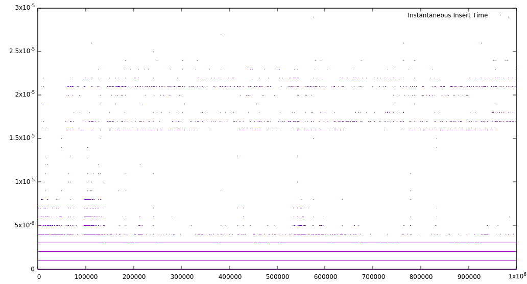
This is certainly a strange looking graph indeed, and that is mostly related to the nature of a splay tree. My guess is that the straight lines represent operations close to each other, and therefore very fast. The much slower insertion times represent operations very far from previous ones, which then become fast due to the splay operation. This is not bad for a worst case, but not particularly impressive either. Things get interesting if we take a look at a different quantity.
Inserting characters randomly doesn’t give a fair representation of the common use case for most editors. To get a more balanced perspective, I also recorded the average time for each insertion into a table of a certain size. I kept a running total of insertion time, and after each insertion, I divided by the current table size. This reflects the average time for each insertion up to that point. I got the following result:
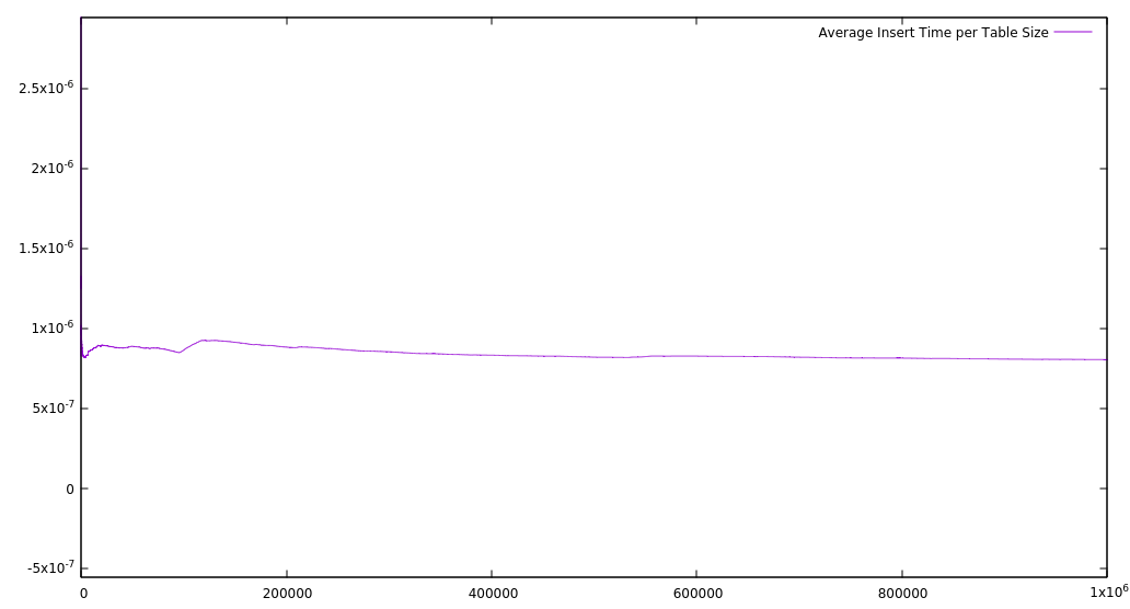
This suggests that, no matter the table size, it should always take about the same time to perform an insertion, and that is a result I’m happy with. As some simple, preliminary tests, there is not much that can be inferred — perhaps a comparison between other implementations (array, linked list, etc) would be interesting. My inner skeptic also feels that running times this quick do seem a bit too good to be true, and there’s always the possibility of a bug that I haven’t noticed. I plan to design some better tests to rule out this possibility.
You can check out all the code on github. My next rough steps are supporting deletions, undo, and then working on an API. After that, multiple cursors, users — and beyond!
This article is also available in Russian thanks to Stanislav
-
I’m using Joaqin’s estimate here ↩