Describing Elliptical Orbits Programmatically
This is a migrated post from my old website. If you see any odd formatting or other inconsistencies, please let me know.
Like most space nerds, I play Kerbal Space Program. I also read The Martian a couple months ago; it was a terrific book, and I highly recommend it. One of my favourite aspects of the book, which is also its claim to fame, is its very impressive intention to be as scientifically accurate as possible. I’ve always been interested in how KSP simulates orbits, but The Martian also got me thinking about how actual orbital maneuvers are planned, and the math involved. That’s why I decided to see if I could use math, and Python, to describe the orbits of Earth and Mars.
The Math
This wikipedia article very helpfully breaks down the math into four distinct steps:
-
Compute the mean anomaly: \(M = nt, nP = 2\pi\)
\[M = \frac{2\pi t}{P}\]Where \(n\) is the mean motion, \(M\) is the mean anomaly, and \(t\) is the time since perihelion. It’s interesting to note that in the consolidated formula, we get the relationship \(\frac{t}{P}\). Therefore, since \(2\pi\) is constant, the term which defines \(M\) is simply the ratio between time since perihelion and the orbital period. This means that any unit of time can be used, as long as it is used for both parameters.
-
Compute the eccentric anomaly \(E\) by solving Kepler’s equation:
\[M = E - \varepsilon\sin{E}\]Where \(\varepsilon\) is the eccentricity of the orbit.
-
Compute the true anomaly \(\theta\) by the equation:
\[(1 - \varepsilon)\tan^2{\frac{\theta}{2}} = (1 + \varepsilon)\tan^2{\frac{E}{2}}\] -
Compute the heliocentric distance:
\[r = a(1 - \varepsilon \cos{E})\]Where \(a\) is the semi-major axis.
Next, we’ll translate each step in to code.
You can find all the code in one place at the end of this article
Step One
First, you’ll need to import the math module, and install matplotlib. I recommend using a package manager to install matplotlib, eg sudo apt-get install python-matplotlib. As the first thing in your file, you should end up with:
import math
from matplotlib import pyplot as plt
For step one, we need to compute the mean anomaly. We need time since perihelion and the orbital period, so we’ll make those parameters:
def step_one(t, p):
	"""
	M = mean anomaly
	M = 2pi * t
	    -------
	       P
	"""
	return (2 * math.pi * t) / p
Step Two
In step two, we’re solving for the eccentric anomaly, and we need the mean anomaly and eccentricity to do it.
Since Kepler’s equation is transcendental, and cannot be solved algebraically, the solution has to be found numerically.
We’ve got two lines, one horizontal, one slanted with slope = 1, and the point where they intersect is our solution. Or, you could move the \(M\) over to get \(M - E + \varepsilon\sin{E} = 0\) and say the root is your solution. I choose the former. It looks something like this:
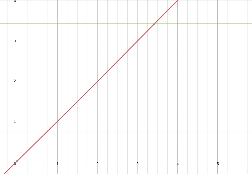
We know that \(M\), a constant value, will always be greater than \(E - \varepsilon\sin{E}\) when \(E = 0\). In fact, the right side of the equation is basically a slanted \(\sin{x}\) graph. You could also think of it as a \(y = x\) graph being sinusoidally translated up and down, where the amplitude of translation is the eccentricity of the orbit.
Knowing that the right side of the equation will always start out as being less than the left, to find the intersection point we can just increase values of \(E\) (starting with \(E = 0\)) until the right side is equal to the left. However: we’ll be computing thousands of positions, and we want to be able to find the solution very quickly, but also with lots of precision. That’s why our algorithm should be as follows:
Initial Conditions: \(E = 0\)
- Is right side \(<\) left side?
- Yes: increment \(E\) by \(1\)
- No: Is right side > left side?
- Yes: decrement \(E\) by \(0.00001\)
- No: stop
This method is fast, but can also be arbitrarily precise by adding as many decimal points to the decrement step as need.
def step_two(m, e):
	"""
	M = mean anomaly
	E = eccentric anomaly
	e = eccentricity

	M = E - esinE
	"""
	def M(E): return E - (e * math.sin(E))
		E = 0
		while m > M(E):
			E += 1
		while M(E) > m:
			E -= 0.00001
		return E
Step Three
This is, by far, the hardest step to implement. It’s easy to get tripped up because it involves a \(\tan\) equation which has two solutions in a given cycle. This step will require a bit of high school trigonometry.
First of all, the right side of the equation, \((1 + \varepsilon)\tan^2{\frac{E}{2}}\), is a number – all of the variables are known – so let’s forget about it for now.
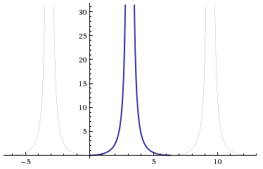
Normally, \(\tan\) has a period of \(\pi\). When you square it, the period doesn’t change, but when you divide the variable \(\theta\) by 2, \(\tan^2{\frac{\theta}{2}}\), then the period becomes \(2\pi\):
Now the right side of our equation, which is a number (not a variable), will be a horizontal line which intersects with the \(\tan^2{\frac{\theta}{2}}\) twice, like this:
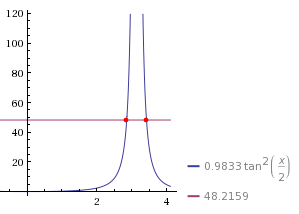
Now the tricky part is that we need both of those solutions. One of the solutions is for when \(0 \le t \le \frac{P}{2}\), and the other is for when \(t \gt \frac{P}{2}\). In other words, without the second solution, you won’t be able to calculate true anomalies for times greater than half the orbital period. My solution is this:
def step_three(e, E):
	"""
	(1 - e)tan^2(theta/2) = (1 + e)tan^2(E/2)
	e = eccentricity
	theta = true anomaly
	E = eccentric anomaly
	"""

	def l(theta): return (1-e)*(math.tan(theta/2))**2

	r = (1+e)*(math.tan(E/2))**2
	theta = 0
	while l(theta) < r:
		theta += 0.1
	while r < l(theta):
		theta -= 0.00001
	return [theta, 2*(math.pi - theta) + theta]
As you can see, this step is very similar in principle to step two, with some key differences. First, I increment by 0.1 and not 1. This is because the angles are very small to begin with, and so incrementing by 0.1 many times is much faster than decrementing by 0.00001 many times. Second, this step returns a list and not a number. The list contains both solutions. In order to get the second solution, a bit of reasoning is need.
First, the \(\tan^2{\frac{\theta}{2}}\) graph is symmetrical in its cycle, meaning the values after \(\pi\) can be described as a reflection of the previous values (\(0 \lt x \lt \pi\)) over a line \(x = \pi\). This means that the distance from the first solution \(\theta_1\) to \(\pi\), which is \(\pi - \theta_1\), is equal to the distance from the second solution \(\theta_2\) to \(\pi\). Therefore, the distance between solutions is \(2(\pi - \theta_1)\). The value of \(\theta_2\) can then be found by the equation:
\[\theta_2 = 2(\pi - \theta_1) + \theta_1\]The solution to use will be determined later, since \(t\) and \(P\) are required.
Okay, we made it through the toughest part! It’s all smooth sailing from here.
Step Four
This is where we calculate the heliocentric distance, or the planet’s distance from the sun. It is given by the equation \(r = a(1 - \varepsilon\cos{E})\). We will need the semi-major axis, eccentricity, and eccentric anomaly as parameters:
def step_four(a, e, E):
	"""
	a = semi-major axis
	e = eccentricity
	E = eccentric anomaly

	r = a(1 - ecosE)
	"""
	return a * (1 - (e * math.cos(E)))
Tying it all together
At this point, you have all the tools you need to predict the position of a planetary body as a function of time. However, I would recommend creating one last function that handles the order of calculations and determines which true anomaly solution to use. I just made a simple, barebones one:
def calculate(e, t, p, a):
	M = step_one(t, p)
	E = step_two(M, e)
	if list(math.modf(float(t) / p))[0] > 0.5:
		theta = step_three(e, E)[1]
	if list(math.modf(float(t) / p))[0] < 0.5:
		theta = step_three(e, E)[0]
	r = step_four(a, e, E)
	return [theta, r]
Lastly, I like to plot things, and I want to plot orbits. At the beginning of this article I said I wanted to predict the orbits of Earth and Mars, so here’s some example code to accomplish this:
e_theta, e_r = [], []
m_theta, m_r = [], []
for x in range(0, 365):
	e_coords = calculate(0.0167, x, 365, 1.496E8)
	e_theta.append(e_coords[0])
	e_r.append(e_coords[1])
	m_coords = calculate(0.0935, x, 687, 2.2792E8)
	m_theta.append(m_coords[0])
	m_r.append(m_coords[1])
plt.polar(e_theta, e_r)
plt.polar(m_theta, m_r, 'r')
plt.show()
This gives me a pretty graph that looks like this:
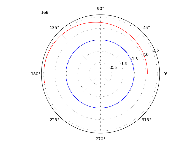
Conclusion
With this code, I see many interesting avenues of research. I can plot more planets, graph their velocity, relative distances, relative angles, etc. Eventually I plan to refine this code for actual calendar dates, and use it to determine launch dates and windows.
Improvements
Some possible improvements could be made on the true anomaly function. Since orbits are quite often plotted one way, and sequentially, it could be optimized for this purpose by accepting the previously calculated angle as a starting point for calculating the next, instead of starting from 0 for all angles. This would be easily done with a parameter which defaults to 0.
The orbits could also be more precise by taking the gravitational influence of other bodies in to account. Additionally, when calculating relative distances more precision could be gained by taking into account the third dimension. This would require additional orbital elements, namely the orbital inclination.
The whole !#
Here’s all the code, for those who are lazy:
import math
from matplotlib import pyplot as plt

def step_one(t, p):
	"""
	M = mean anomaly
	M = 2pi * t
	    -------
	       P
	"""
	return (2 * math.pi * t) / p

def step_two(m, e):
	"""
	M = mean anomaly
	E = eccentric anomaly
	e = eccentricity

	M = E - esinE
	"""
	def M(E): return E - (e * math.sin(E))
	E = 0
	while m > M(E):
		E += 1
	while M(E) > m:
		E -= 0.00001
	return E

def step_three(e, E):
	"""
	(1 - e)tan^2(theta/2) = (1 + e)tan^2(E/2)
	e = eccentricity
	theta = true anomaly
	E = eccentric anomaly
	"""
	def l(theta): return (1-e)*(math.tan(theta/2))**2
	r = (1+e)*(math.tan(E/2))**2
	theta = 0
	while l(theta) < r:
		theta += 0.1
	while r < l(theta):
		theta -= 0.00001
	return [theta, 2*(math.pi - theta) + theta]

def step_four(a, e, E):
	"""
	a = semi-major axis
	e = eccentricity
	E = eccentric anomaly

	r = a(1 - ecosE)
	"""
	return a * (1 - (e * math.cos(E)))

def calculate(e, t, p, a):
	M = step_one(t, p)
	E = step_two(M, e)
	if list(math.modf(float(t) / p))[0] > 0.5:
		theta = step_three(e, E)[1]
	if list(math.modf(float(t) / p))[0] < 0.5:
		theta = step_three(e, E)[0]
	r = step_four(a, e, E)
	return [theta, r]

e_theta, e_r = [], []
m_theta, m_r = [], []
for x in range(0, 365):
	e_coords = calculate(0.0167, x, 365, 1.496E8)
	e_theta.append(e_coords[0])
	e_r.append(e_coords[1])
	m_coords = calculate(0.0935, x, 687, 2.2792E8)
	m_theta.append(m_coords[0])
	m_r.append(m_coords[1])
plt.polar(e_theta, e_r)
plt.polar(m_theta, m_r, 'r')
plt.show()
Final Thoughts
If you made it all the way to the end, I’m very impressed. Thanks for reading!
I try to be as accurate as possible, but if you see any mistakes or have any questions, comment below or feel free to email me.